Chapter 6 Exploring isoforms of interest
One of the most powerful aspects of long-read single-cell sequencing is its ability to profile isoform-specific information at single-cell resolution. This capability opens up numerous avenues for analysis. In our lab we are interested in exploring the role of RNA isoforms in neuronal differentiation and there are many examples in the literature of isoforms regulating this process. We will cover some very general analysis with this focus in mind.
6.1 Isoforms expressed per gene
With long-read single-cell data, we have the ability to analyze all the isoforms expressed by a given gene. In our data we can see that most genes express more than one isoform.
Code
# let's aggregate the expression data by cell type
counts <- AggregateExpression(
  seu_obj,
  assays = "iso",
  return.seurat = FALSE,
  group.by = "sctype_db"
)

as.data.frame(counts) -> df
row.names(df) -> df$gene

#split transcript ids into gene and transcript id
pseudobulk_data <- df %>% separate(gene, into = c("transcript_id", "gene_id"), sep = "-",  extra = "merge")
#df$transcript_id <- sub("\\..*", "", df$transcript_id)

# 2. Count the number of isoforms per gene
isoform_count_per_gene <- pseudobulk_data %>%
  group_by(gene_id) %>%
  summarise(n_isoforms = n_distinct(transcript_id))

# 3. count isoforms per category
isoform_count_per_gene <- isoform_count_per_gene %>%
  mutate(isoform_category = case_when(
    n_isoforms == 1 ~ "1",
    n_isoforms >= 2 & n_isoforms <= 3 ~ "2-3",
    n_isoforms >= 4 & n_isoforms <= 5 ~ "4-5",
    n_isoforms >= 6 ~ "6+"
  ))


# 4. Calculate the percentage of genes in each bin
isoform_count_summary <- isoform_count_per_gene %>%
  dplyr::count(isoform_category) %>%
  mutate(percent = (n / sum(n)) * 100)

ggplot(isoform_count_summary, aes(x = isoform_category, y = percent)) +
  geom_bar(stat = "identity", fill = "lightblue", color = "black") +
  labs(title = "Number of Isoforms per Gene",
       x = "Isoforms per Gene",
       y = "Genes, %") +
  theme_minimal() +
  theme(legend.position = "none",
        plot.title = element_text(hjust = 0.5))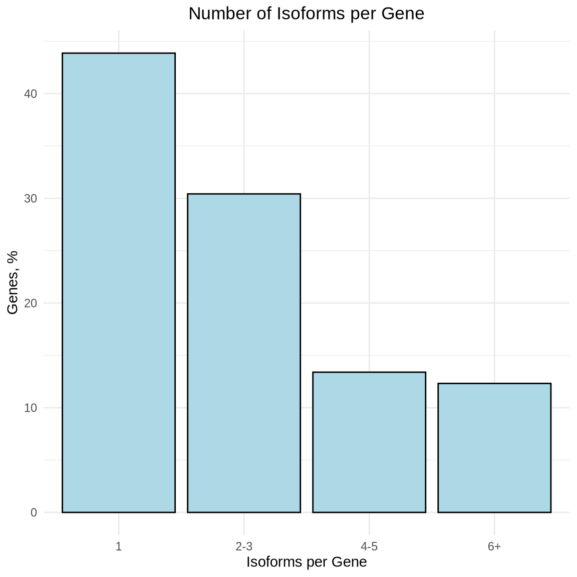
6.2 Top 10 Genes with Most Isoforms
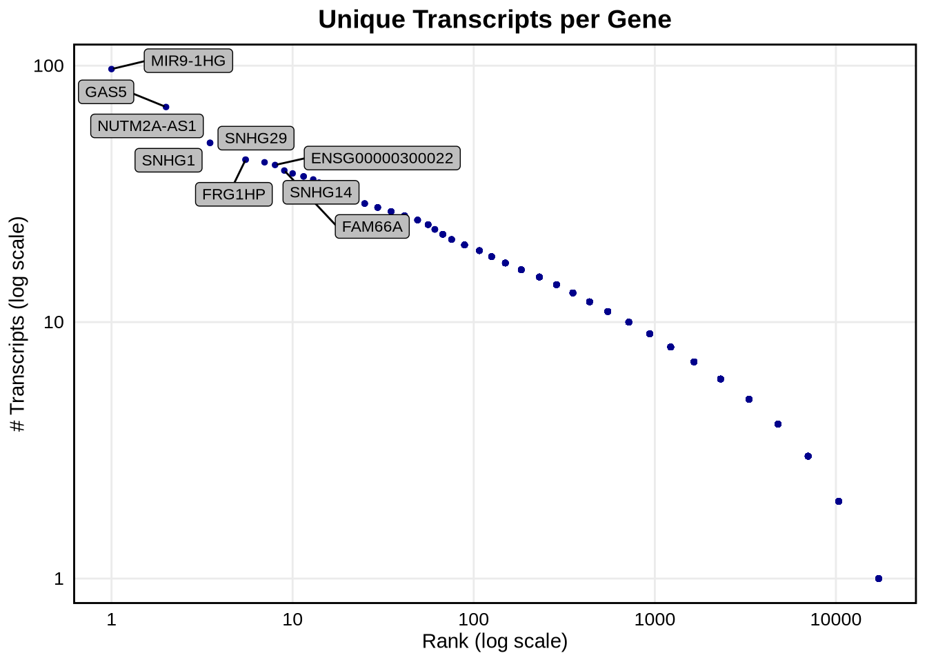
We can see that about 45% of genes express a single isoform, however there are some genes like MIR9-1HG that have a lot of unique isoforms, 97 in fact. The top 10 genes with the most isoforms are listed below.
Code
# Genes ranked by the number of transcript isoforms detected across all samples
gene_transcript_counts <- pseudobulk_data %>%
  group_by(gene_id) %>%
  summarise(unique_transcripts = n_distinct(transcript_id)) %>%
  arrange(desc(unique_transcripts))

# Select the top 10 genes based on unique transcript counts
top10 <- gene_transcript_counts %>% top_n(10, unique_transcripts)

top10
## # A tibble: 10 × 2
## gene_id unique_transcripts
## <chr> <int>
## 1 MIR9-1HG 97
## 2 GAS5 69
## 3 NUTM2A-AS1 50
## 4 SNHG1 50
## 5 FRG1HP 43
## 6 TMEM161B-DT 43
## 7 SNHG29 42
## 8 ENSG00000300022 41
## 9 FAM66A 39
## 10 SNHG14 38We can also plot unique transcripts per gene on a log scale showing that the number of isoforms per gene varies across our data.
Code
# Plot ranked genes by unique "BambuTx" transcript count
ggplot(gene_transcript_counts, aes(x = rank(desc(unique_transcripts)), y = unique_transcripts)) +
  geom_point(color = "darkblue", size = 1) +  # Points for each gene

  # Log scale for both axes
  scale_x_log10() +
  scale_y_log10() +

  # Title and labels
  labs(
    title = "Unique Transcripts per Gene",
    x = "Rank (log scale)",
    y = "# Transcripts (log scale)"
  ) +

  # Highlight and label the top 10 genes with gray background and black border around the text
  geom_label_repel(
    data = gene_transcript_counts %>% filter(gene_id %in% top10$gene_id),
    aes(label = gene_id),
    fill = "gray",          # Gray background for the label
    color = "black",         # Black text color
    label.size = 0.25,       # Border thickness around the label
    label.r = unit(0.15, "lines"),  # Border radius (rounded corners)
    size = 3,
    box.padding = 0.2,
    max.overlaps = 14
  ) +

  # Minimal theme and additional styling
  theme_minimal() +
  theme(
    plot.title = element_text(size = 14, face = "bold", hjust = 0.5), # Centered title
    axis.text = element_text(size = 10, color = "black"),             # Black axis tick labels
    axis.title = element_text(color = "black"),                       # Black axis titles
    panel.grid.minor = element_blank(),
    panel.border = element_rect(color = "black", fill = NA, linewidth = 1)  # Black border around the graph
  )
6.3 Exploring MACF1 isoforms
We are interested in isoforms that regulate neuronal differentiation, we can look at some genes of interest. Let’s look at gene MACF1. The gene seems to play some important role in neural migration which is not fully understood yet. First let’s try and visualize the expression of these isoforms on a UMAP to see if we can uncover anything interesting. MACF1 has 35 expressed isoforms so let’s only plot the top 12 most highly expressed.
Code
features <- rownames(filt_seurat_object@assays$iso@features)

# Define the gene of interest
gene <- "MACF1"

# Access the data matrix for the 'iso' assay
expression_matrix <- GetAssayData(filt_seurat_object, assay = "iso", slot = "data")

# Filter features containing the gene name
matching_features <- grep(paste0("(^|-|\\b)", gene, "($|\\b)"), rownames(expression_matrix), value = TRUE)

# Subset the expression matrix to include only the matching features
subset_expression <- expression_matrix[matching_features, , drop = FALSE]

# Calculate the total expression for each matching feature
total_expression <- Matrix::rowSums(subset_expression)

# Rank features by average expression
top_features <- names(sort(total_expression, decreasing = TRUE))

# Print the ranked features (optional)
print(data.frame(Feature = top_features, Expression = total_expression[top_features]))
## Feature Expression
## ENST00000361689.7-MACF1 ENST00000361689.7-MACF1 143.862407
## ENST00000289893.8-MACF1 ENST00000289893.8-MACF1 62.133601
## ENST00000372925.6-MACF1 ENST00000372925.6-MACF1 45.932634
## ENST00000372915.8-MACF1 ENST00000372915.8-MACF1 45.461522
## ENST00000567887.5-MACF1 ENST00000567887.5-MACF1 45.092944
## ENST00000686657.1-MACF1 ENST00000686657.1-MACF1 44.609476
## ENST00000564288.6-MACF1 ENST00000564288.6-MACF1 40.689721
## ENST00000524432.5-MACF1 ENST00000524432.5-MACF1 27.310250
## ENST00000686687.1-MACF1 ENST00000686687.1-MACF1 19.939477
## ENST00000497964.1-MACF1 ENST00000497964.1-MACF1 17.945311
## ENST00000530275.3-MACF1 ENST00000530275.3-MACF1 16.728830
## ENST00000691623.1-MACF1 ENST00000691623.1-MACF1 14.286232
## ENST00000602528.2-MACF1 ENST00000602528.2-MACF1 13.942571
## ENST00000687271.1-MACF1 ENST00000687271.1-MACF1 12.934634
## ENST00000476350.1-MACF1 ENST00000476350.1-MACF1 12.210176
## ENST00000496804.5-MACF1 ENST00000496804.5-MACF1 12.181141
## ENST00000686067.1-MACF1 ENST00000686067.1-MACF1 10.238947
## ENST00000690080.1-MACF1 ENST00000690080.1-MACF1 8.279051
## ENST00000497807.1-MACF1 ENST00000497807.1-MACF1 8.021857
## ENST00000693209.1-MACF1 ENST00000693209.1-MACF1 7.429056
## ENST00000693392.1-MACF1 ENST00000693392.1-MACF1 7.317640
## ENST00000472385.2-MACF1 ENST00000472385.2-MACF1 7.075353
## ENST00000602421.5-MACF1 ENST00000602421.5-MACF1 6.698620
## ENST00000686260.1-MACF1 ENST00000686260.1-MACF1 6.297806
## ENST00000688426.1-MACF1 ENST00000688426.1-MACF1 6.232290
## ENST00000687997.1-MACF1 ENST00000687997.1-MACF1 6.056226
## ENST00000690939.1-MACF1 ENST00000690939.1-MACF1 5.445340
## ENST00000683517.1-MACF1 ENST00000683517.1-MACF1 3.526815
## ENST00000442046.5-MACF1 ENST00000442046.5-MACF1 3.018726
## ENST00000689911.1-MACF1 ENST00000689911.1-MACF1 2.657853
## ENST00000484793.5-MACF1 ENST00000484793.5-MACF1 2.181164
## ENST00000467673.5-MACF1 ENST00000467673.5-MACF1 2.131094
## ENST00000686941.1-MACF1 ENST00000686941.1-MACF1 1.058887
## ENST00000672812.1-MACF1 ENST00000672812.1-MACF1 1.055652
## ENST00000528611.1-MACF1 ENST00000528611.1-MACF1 0.401423Code
options(repr.plot.width=12, repr.plot.height=12)
# Plot the top 16 features in descending order of their average expression
plots <- FeaturePlot(
  filt_seurat_object,
  features = head(top_features, 12),
  reduction = "umap",
  order = TRUE, # Ensures higher-expressing cells are plotted on top
  pt.size = 1)

# Adjust title size for each plot
plots <- lapply(plots, function(plot) {
  plot + theme(plot.title = element_text(size = 8))
})

# Combine the adjusted plots
CombinePlots(plots = plots, ncol = 3)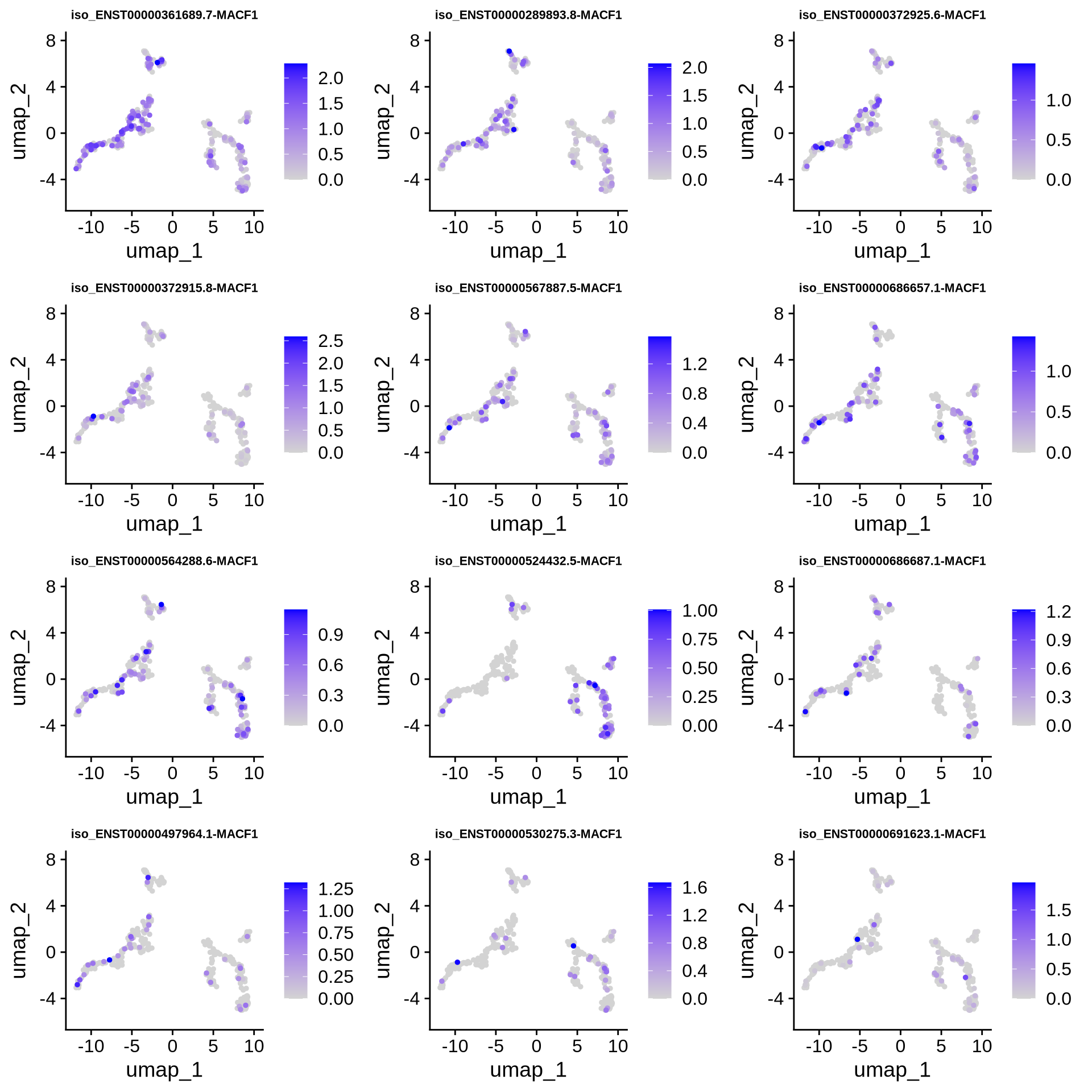
6.4 Expression of MACF1 isoforms Across Cell Types
Let’s look at isoforms ENST00000564288.6, ENST00000361689.7, ENST00000289893.8 and ENST00000524432.5 in some more detail and plot the normalized expression of these isoforms across each cell type. We can see that the expression of ENST00000524432.5 shows a cell type specific profile.
Code
features_MACF1 <- c("ENST00000564288.6-MACF1", # canonical
                    "ENST00000361689.7-MACF1", # most cell types
                    "ENST00000289893.8-MACF1", # most cell types
                    "ENST00000524432.5-MACF1") # radial glia

VlnPlot(seu_obj, features = features_MACF1, ncol = 2)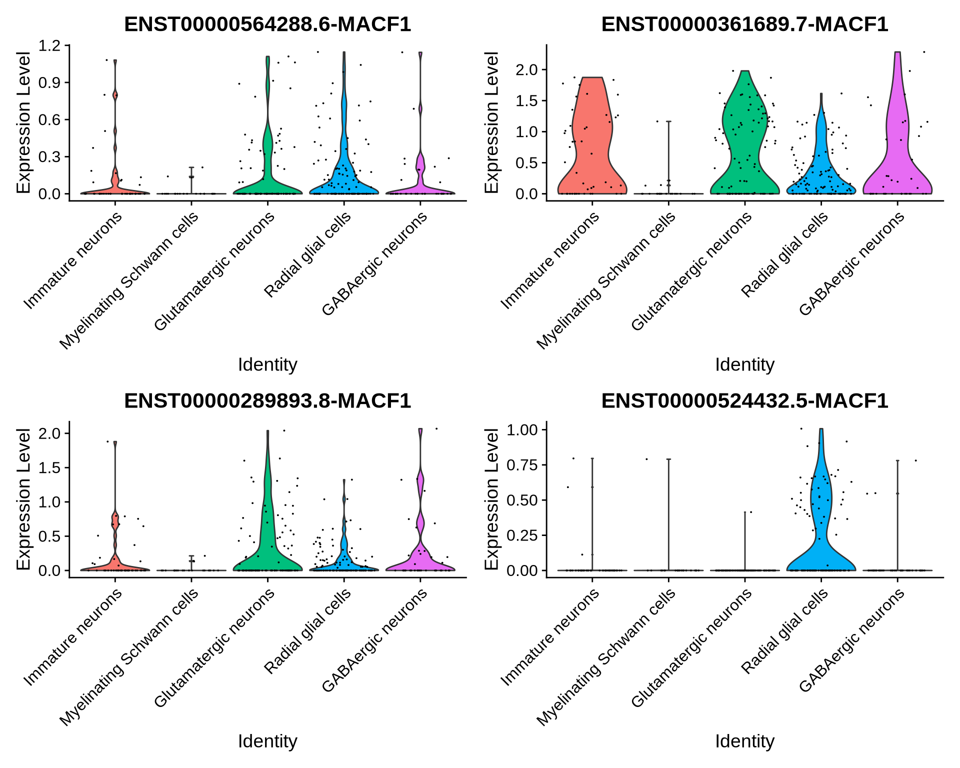
We can also show this enrichment with a dotplot.
Code
dittoDotPlot(seu_obj, vars = features_MACF1, group.by = "sctype_db", scale = FALSE)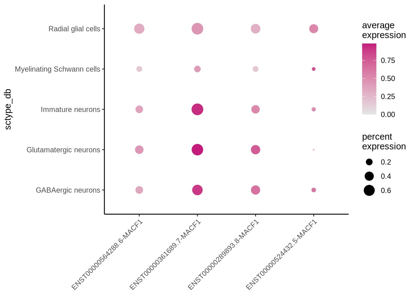
let’s look at our DE results comparing glutamatergic neurons and Radial glia cells that we calculated in the previous chapter and filter for significant MACF1 isoforms. If we plot these features on a Volcano plot we see isoform ENST00000524432.5 is enriched in radial glia cells. In fact its enrichment compared to glutamatergic neurons is pretty high with a Log2fold change of 4.16.
Code
glu_RG_iso %>%
  rownames_to_column("isoform") %>%
  filter(grepl("MACF1", isoform)) %>%
  filter(p_val_adj < 0.5)
## isoform p_val avg_log2FC pct.1 pct.2 p_val_adj
## 1 ENST00000524432.5-MACF1 1.025842e-10 -4.163237 0.011 0.384 6.539231e-06Code
EnhancedVolcano(glu_RG_iso, lab=rownames(glu_RG_iso),
                x='avg_log2FC', y='p_val_adj',
                #selectLab= "VIM",
                pCutoff=0.05, FCcutoff=2,
                selectLab = "ENST00000524432.5-MACF1",
                boxedLabels = TRUE,
                drawConnectors = TRUE,
                title = "ENST00000524432.5-MACF1 is upregulated \n in Radial glial Cells compared to Glutamatergic Neurons")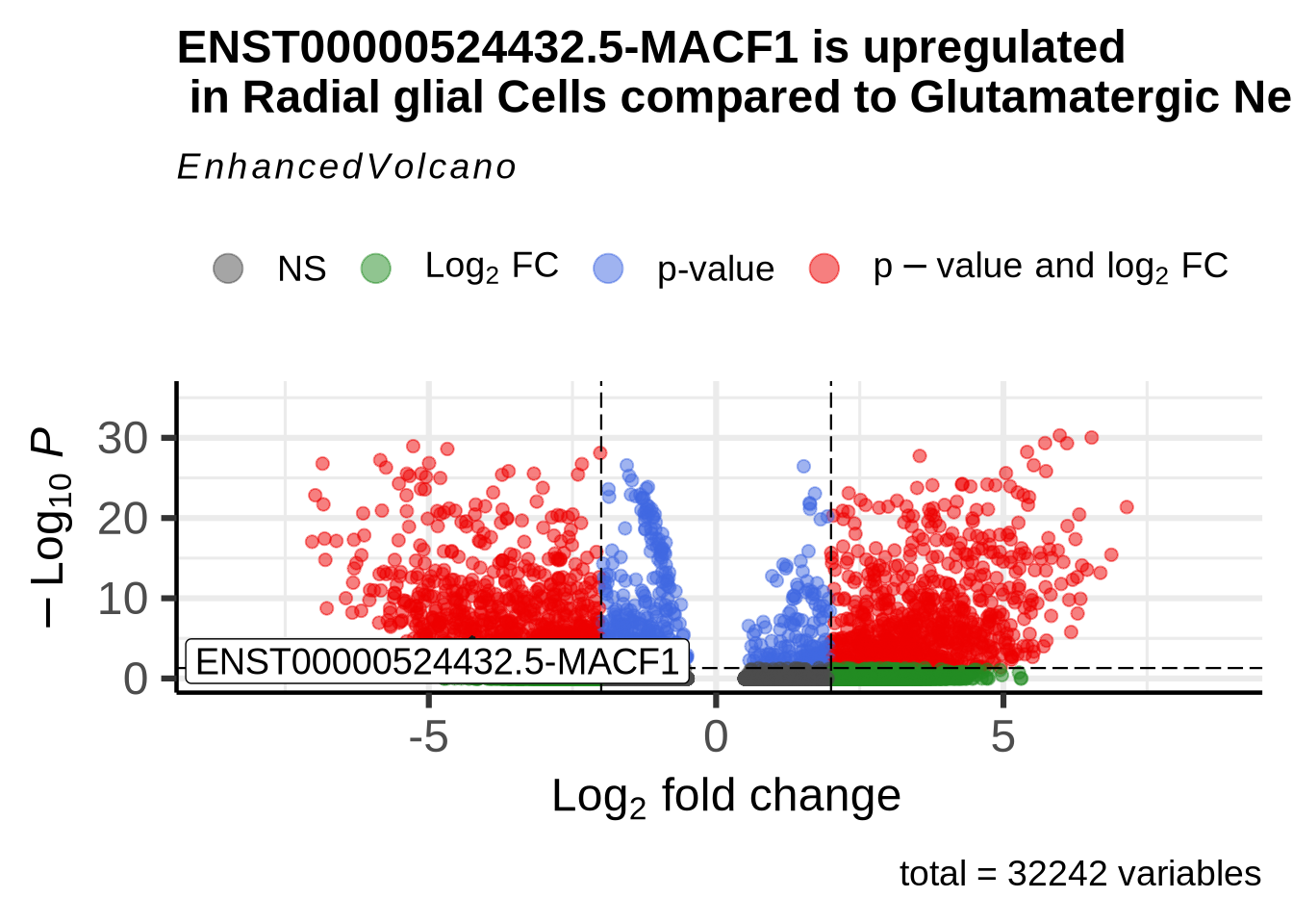
6.5 Visualization of Isoform Structures
Now that we know some MACF1 isoforms expression is significantly different in these two cell populations it may be of interest to visualize the isoform structures. This analysis will help us explore the similarities and differences between our isoforms of interest.
There are many visualization options available to us and many of these are available in R. In fact FLAMES has its own visualization function FLAMES::plot_isoform_reduced_dim. This function is designed to work on single cell experiment object and not Seurat object. Although it is possible to switch between these formats, for the purpose of this tutorial we want to keep file conversations to a minimum to keep the analysis simple.
We instead recommend using IsoVis (Wan et al., 2024), which was developed in the Clark Lab. The tool is a web application specifically designed for visualizing isoform structures. This visualization can provide valuable insights into the potential functions of different isoforms.
First let’s prepare the count data that we will load into Isovis1
Code
#extract some isoform expression data to visualize in IsoVis
#use pseudobulk counts we got from above
pseudobulk_data -> pseudobulk_data_IsoVis_format
row.names(pseudobulk_data_IsoVis_format) <- NULL

write.csv(pseudobulk_data_IsoVis_format, "output_files/Pseudobulk_exp.csv", row.names = FALSE)
To use IsoVis click on the following link https://isomix.org/isovis/ and upload the isoform_annotated.gtf file located in the FLAMES output dir and Pseudobulk_exp.csv generated above. For more detail on how to use IsoVis click the ‘IsoVis tutorial’ button or read the publication.
Embedded below is the figure generated by IsoVis2. Here we we will visualise our 4 isoforms of interest. We can see MACF1 is a very complex gene with many exons, a variety of alternative transcription start sites. Structural visualization aids in identifying critical variations such as alternative splicing events, unique protein-coding regions, and functional domains.
Code
knitr::include_graphics("images/IsoVis_ENSG00000127603.png")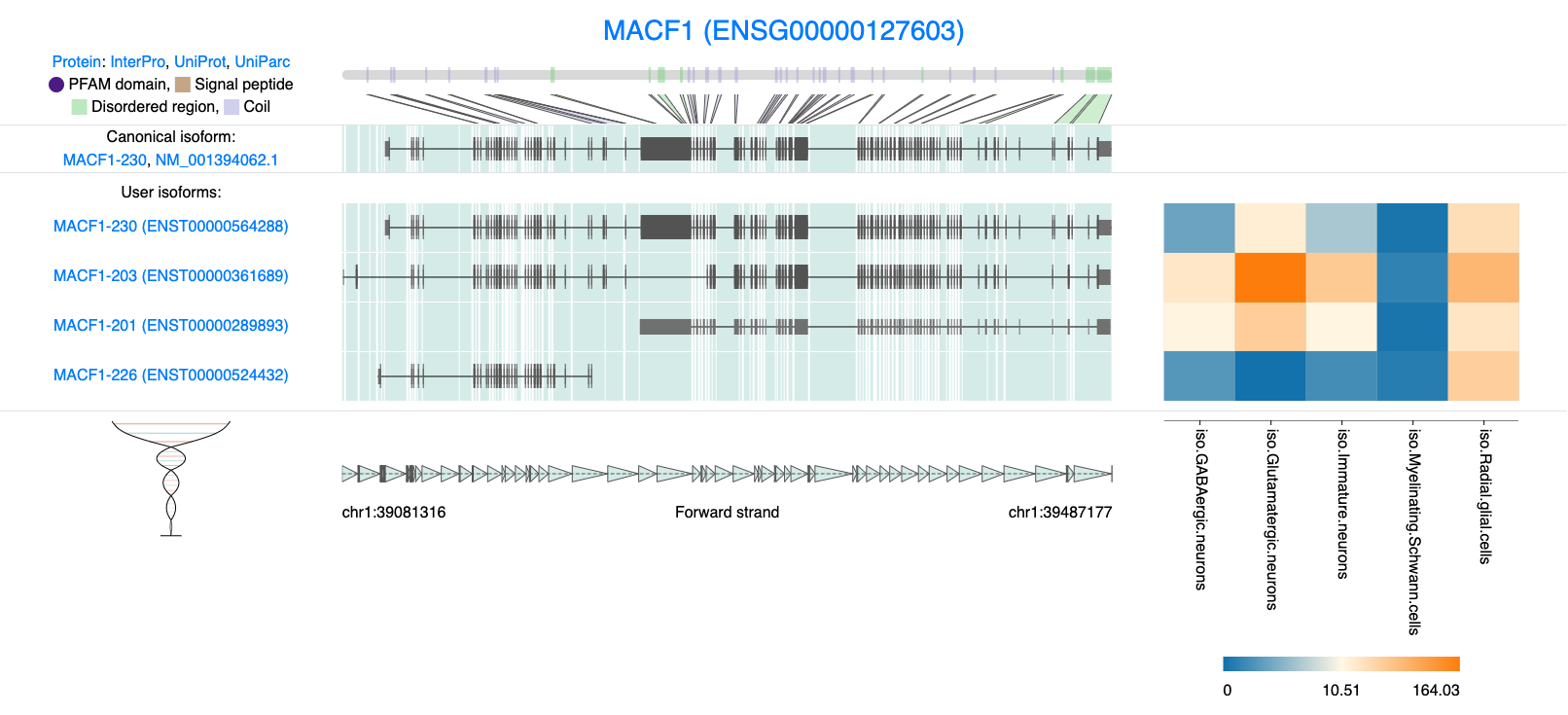
Figure 6.1: IsoVis visualization of 4 MACF1 isoforms.
Our pseudobulk expression data clearly demonstrates that ENST00000524432.5 is predominantly expressed in radial glia cells. This isoform is particularly interesting, as it is significantly shorter than others and lacks many of the protein domains present in ENST00000564288.6 (the canonical isoform). Notably, all four isoforms exhibit different transcription start sites (TSS), suggesting that TSS variation may be linked to cell-type-specific expression or distinct proteaforms
For example, ENST00000289893.8 shows comparably high expression levels across most cell types. However, a deeper exploration of this isoform reveals that it does not produce a functional protein. This is evident from examining the Ensembl data, accessible via the isoform hyperlink, where we can see that no open reading frames (ORFs) are associated with this transcript.
There are lots of additional analysis that could be performed to further explore the function of our MACF1 isoforms, these include domain enrichment analysis and protein folding to name a few.
Please be careful when interpreting pseudubulk expression data. Although the data can give you some indication of relative expression across cell types, this numbers can be affected by the number of cells in each cluster.↩︎
When Viewing this data in the web browser users will have more functionality. This includes a zoom function, looking at protein domains and rearranging isoform tracks and known visualizing open reading frames.↩︎