Chapter 7 Isoform Classification
7.1 Classification with SQANTI
In the previous Chapter we looked at some genes of interest like MCAF1 and some of the isoforms related to this gene. As you can see MCAF1 is a highly complex gene with many exons, varied Transcription start sites and many splice junctions. Evaluating this information manually for each isoform is complex and time consuming. A tool that that is very useful here is SQANTI3 (Pardo-Palacios et al., 2024) which will categorize our isoforms3 and determine whether they are coding or non-coding.
If you install SQANTI3 and run the following command in your FLAMES output folder you will generate a classifications.txt file. This output file is located in the data folder on the github page. SQANTI can also generate an HTML report with lots of figures summarizing your isoforms which can be very helpful. We will do something similar but instead plot this information stratified by cell type.
Code
GTF="gencode.v47.annotation.gtf"
genome="genome.fa"
#filter gtf file to remove annotation of unknown strands
awk '$7 == "+" || $7 == "-"' isoform_annotated.gtf > remove_unknownstrand.gtf
#run SQANTIpython3
#you may need need to activate a conda environment
SQANTI3-5.2.1/sqanti3_qc.py remove_unknownstrand.gtf ${GTF} ${genome}
If we examine the classifications file, we can see that each isoform in our GTF file has been categorized based on its structural characteristics, coding potential, and additional attributes.
Code
SQANTI <- read.csv("data/remove_unknownstrand_classification.txt", sep ='\t')
#SQANTI$isoform <- sub("\\..*", "", SQANTI$isoform) # remove numbers after .

head(SQANTI, 3)
## isoform chrom strand length exons structural_category associated_gene associated_transcript ref_length
## 1 BambuTx1 chr1 + 2381 3 novel_in_catalog ENSG00000294260.1 novel 1694
## 2 BambuTx2 chr1 - 595 2 antisense novelGene_ENSG00000302070.1_AS novel NA
## 3 ENST00000003583.12 chr1 - 2544 8 full-splice_match ENSG00000001460.18 ENST00000003583.12 2544
## ref_exons diff_to_TSS diff_to_TTS diff_to_gene_TSS diff_to_gene_TTS subcategory RTS_stage all_canonical
## 1 2 NA NA -2481 -17 combination_of_known_splicesites FALSE canonical
## 2 NA NA NA NA NA multi-exon FALSE canonical
## 3 8 0 0 0 0 reference_match FALSE canonical
## min_sample_cov min_cov min_cov_pos sd_cov FL n_indels n_indels_junc bite iso_exp gene_exp ratio_exp FSM_class coding
## 1 NA NA NA NA NA NA NA FALSE NA NA NA C non_coding
## 2 NA NA NA NA NA NA NA FALSE NA NA NA A non_coding
## 3 NA NA NA NA NA NA NA FALSE NA NA NA C coding
## ORF_length CDS_length CDS_start CDS_end CDS_genomic_start CDS_genomic_end predicted_NMD perc_A_downstream_TTS seq_A_downstream_TTS
## 1 NA NA NA NA NA NA NA 75 TAAAAAAAAAAAATAAGTGA
## 2 NA NA NA NA NA NA NA 95 AAAAAAAAAAAAAAGAAAAA
## 3 122 369 1009 1377 24358540 24358172 FALSE 15 TATTGAGCTTTTGGGTACCC
## dist_to_CAGE_peak within_CAGE_peak dist_to_polyA_site within_polyA_site polyA_motif polyA_dist polyA_motif_found
## 1 NA NA NA NA NA NA NA
## 2 NA NA NA NA NA NA NA
## 3 NA NA NA NA NA NA NA
## ORF_seq
## 1 <NA>
## 2 <NA>
## 3 MSHKVKENSSHQPTLPSVPRTFLRRRPIMSVAADNLGGGSTTLAWHPSRTAAIAFVLSWRHCSLETSPQPHRLQWLPEQKGGVDRAPWLLPHAPIQAAFRHDSLPQTEGTPEAQTSRRISPP
## ratio_TSS
## 1 NA
## 2 NA
## 3 NAThere is a lots information one can extract from the classifications.txt file. to get a more complete picture of the isoforms in the sample Lets plot some of this information.
Code
#we can use the pseudobulk_data counts calculated previously
# Select cell type columns and gather into long format
long_data <- pseudobulk_data %>%
  pivot_longer(
    cols = starts_with("iso."),
    names_to = "cell_type",
    values_to = "expression"
  )

# Filter for non-zero expression to identify genes and isoforms expressed in each cell type
filtered_data <- long_data %>%
  filter(expression > 0) %>%
  dplyr::select(cell_type, transcript_id, gene_id) %>%
  distinct()

# Calculate unique gene and isoform counts for each cell type
cell_type_summary <- filtered_data %>%
  group_by(cell_type) %>%
  summarise(
    num_genes = n_distinct(gene_id),
    num_isoforms = n_distinct(transcript_id)
  ) %>%
  pivot_longer(cols = c(num_genes, num_isoforms),
               names_to = "Category",
               values_to = "Count")

# Plot the data
p1 <- ggplot(cell_type_summary, aes(x = cell_type, y = Count, fill = Category)) +
  geom_bar(stat = "identity", position = "dodge", color = "black", width = 0.8) +
  theme_minimal() +
  labs(title = "Number of genes and isoforms \n per cell type",
       x = "Cell Type",
       y = "Count") +
  theme(
    plot.title = element_text(size = 20, face = "bold", hjust = 0.5),
    axis.title.x = element_text(size = 14),
    axis.title.y = element_text(size = 14),
    axis.text.x = element_text(size = 12, angle = 45, hjust = 1),
    axis.text.y = element_text(size = 12),
    legend.title = element_blank()
  )


# plot the structural category per cell type
  merged_data <- merge(pseudobulk_data, SQANTI,
                     by.x = "transcript_id",
                     by.y = "isoform",
                     all.x = TRUE)

  # Pivot pseudobulk data to long format for cell types
long_data <- merged_data %>%
  pivot_longer(
    cols = starts_with("iso."),
    names_to = "cell_type",
    values_to = "expression"
  )

# Generate outr new df thatw e can use for plotting attributes deffiend by cell type
filtered_data <- long_data %>%
  filter(expression > 0) %>%
  distinct()

# Calculate unique counts of genes and isoforms per structural category and cell type
category_summary <- filtered_data %>%
  group_by(cell_type, structural_category, subcategory, coding) %>%
  summarise(
    num_genes = n_distinct(gene_id),
    num_isoforms = n_distinct(transcript_id),
    .groups = "drop"
  )

# Plot number of isoforms per structural category for each cell type
p2 <- ggplot(category_summary, aes(x = cell_type, y = num_isoforms, fill = structural_category)) +
  geom_bar(stat = "identity", position = "stack", width = 0.8) +
  theme_minimal() +
  labs(
    title = "Isoforms by structural category \n across cell types",
    x = "Cell Type",
    y = "Number of Isoforms",
    fill = "Structural Category"
  ) +
  theme(
    plot.title = element_text(size = 20, face = "bold", hjust = 0.5),
    axis.title.x = element_text(size = 14),
    axis.title.y = element_text(size = 14),
    axis.text.x = element_text(size = 12, angle = 45, hjust = 1),
    axis.text.y = element_text(size = 12),
    legend.title = element_text(size = 14),
    legend.text = element_text(size = 12)
  )

p3 <- ggplot(category_summary, aes(x = cell_type, y = num_isoforms, fill = subcategory)) +
  geom_bar(stat = "identity", position = "stack", width = 0.8) +
  theme_minimal() +
  labs(
    title = "Isoforms by structural subcategory \n across cell types",
    x = "Cell Type",
    y = "Number of Isoforms",
    fill = "subcategory"
  ) +
  theme(
    plot.title = element_text(size = 20, face = "bold", hjust = 0.5),
    axis.title.x = element_text(size = 14),
    axis.title.y = element_text(size = 14),
    axis.text.x = element_text(size = 12, angle = 45, hjust = 1),
    axis.text.y = element_text(size = 12),
    legend.title = element_text(size = 14),
    legend.text = element_text(size = 12)
  )


p4 <- ggplot(category_summary, aes(x = cell_type, y = num_isoforms, fill = coding)) +
  geom_bar(stat = "identity", position = "fill", width = 0.8) +
  theme_minimal() +
  labs(
    title = "Proportion of coding isoforms \n across cell types",
    x = "Cell Type",
    y = "Proportion of Isoforms",
    fill = "Structural Category"
  ) +
  scale_y_continuous(labels = scales::percent) +  # This will show y-axis as percentages
  theme(
    plot.title = element_text(size = 20, face = "bold", hjust = 0.5),
    axis.title.x = element_text(size = 14),
    axis.title.y = element_text(size = 14),
    axis.text.x = element_text(size = 12, angle = 45, hjust = 1),
    axis.text.y = element_text(size = 12),
    legend.title = element_text(size = 14),
    legend.text = element_text(size = 12)
  )


#Plots

cowplot::plot_grid(p1, p2, p3, p4, ncol = 2)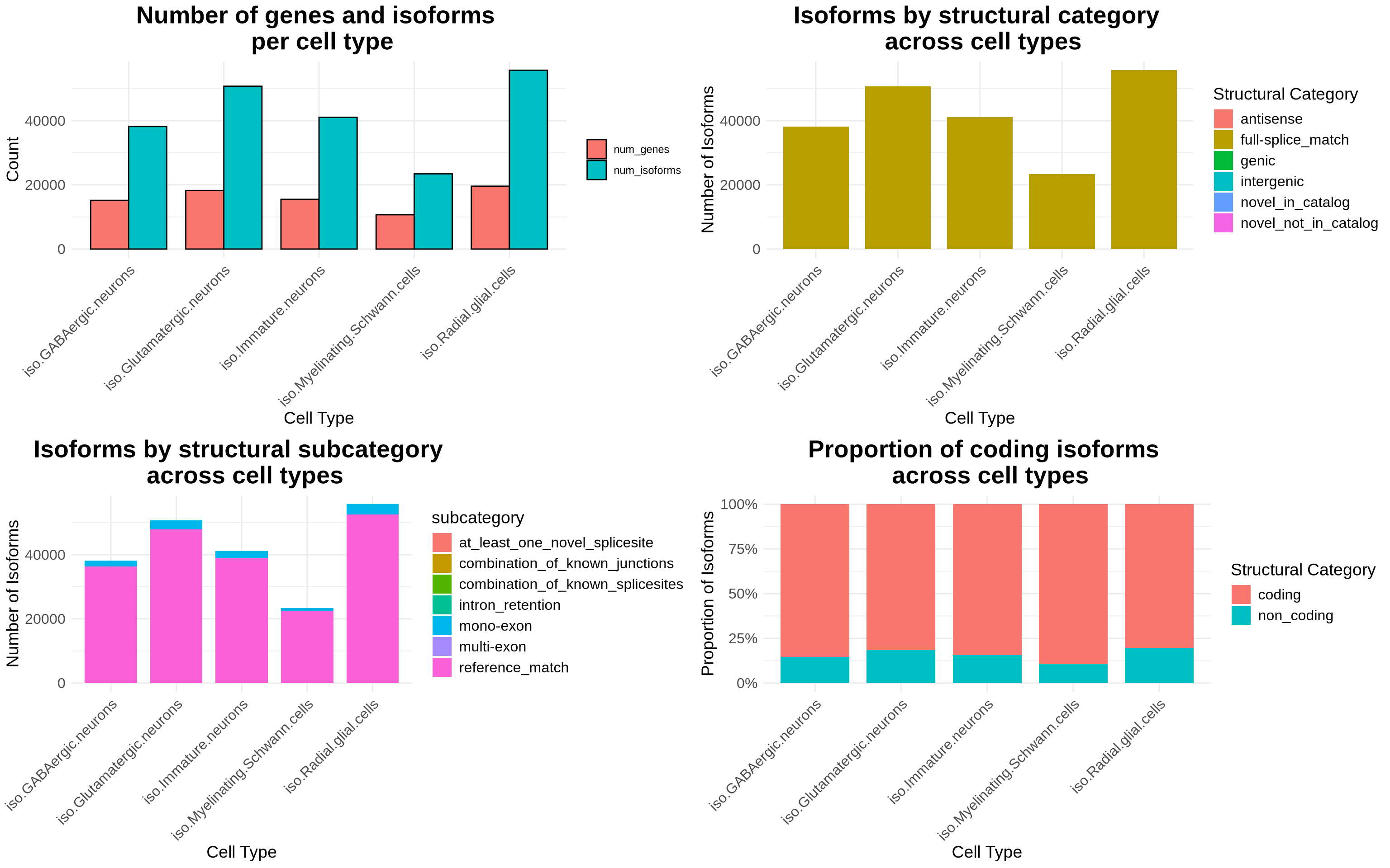
7.2 Cell type specific isoforms
We can also look at isoforms that are unique to each Cell type. We define unique as an isoforms that has 5 or more counts in one cell type and ≤ 1 count in all other cell types. Users can adjust the thresholds mentioned below4.
Code
# Filter the data based on the expression cutoff
# Set expression cutoff threshold
expression_cutoff <- 5
max_expression_in_all_other_cells_types = 1

# Filter isoforms based on the new criteria
exclusive_isoforms <- long_data %>%
  group_by(transcript_id) %>%
  filter(
    # Only one cell type where expression > cutoff
    sum(expression > expression_cutoff) <= 1,
    # Ensure all other cell types have 0 expression
    all(expression < max_expression_in_all_other_cells_types | expression > expression_cutoff)
  ) %>%
  ungroup()

# Count the unique isoforms per cell type
# Adjust counting logic
exclusive_isoforms_count <- exclusive_isoforms %>%
  group_by(cell_type) %>%
  summarise(
    unique_isoforms = sum(expression > expression_cutoff)  # Count only isoforms with valid expression
  ) %>%
  ungroup()

# Plot the results
ggplot(exclusive_isoforms_count, aes(x = cell_type, y = unique_isoforms, fill = cell_type)) +
  geom_bar(stat = "identity", color = "black", width = 0.8) +
  theme_minimal() +
  labs(
    title = "Number of isoforms unique \n to each cell type",
    x = "Cell Type",
    y = "Number of Unique Isoforms"
  ) +
  theme(
    plot.title = element_text(size = 20, face = "bold", hjust = 0.5),
    axis.title.x = element_text(size = 14),
    axis.title.y = element_text(size = 14),
    axis.text.x = element_text(size = 12, angle = 45, hjust = 1),
    axis.text.y = element_text(size = 12),
    legend.title = element_blank()
  )
These cell type specific isoforms may be particularly interesting to study further, as they likely play important roles in differentiation and cell function. We could extract these isoforms for further analysis.
Lets use another helpful resource to explore these cell type specific isoforms.
We can use the BioMart (Smedley et al., 2009) package to get some more metadata about each isoform. There is lots of data that can be extracted from BioMart. This is just a simple example of what can be done with this cell type specif data.
Code
library("biomaRt")

exclusive_isoforms_uniq <- exclusive_isoforms %>%
  filter(expression >= max_expression_in_all_other_cells_types) %>%
  arrange(desc(expression))

exclusive_isoforms_uniq$transcript_id <- sub("\\..*", "", exclusive_isoforms_uniq$transcript_id)

# Retrieve gene biotype from Ensembl
  mart <- useMart(biomart = "ensembl",
                 dataset = "hsapiens_gene_ensembl")

  biotype_info_transcript <- getBM(attributes = c("ensembl_transcript_id", "transcript_is_canonical", 'transcript_biotype', 'transcript_length'),
                                   filters = 'ensembl_transcript_id',
                                   values = exclusive_isoforms_uniq$transcript_id,
                                   mart = mart)

  #merge excluive isoforms and biomart data togehter
  merged_biomart_data <- merge(exclusive_isoforms_uniq, biotype_info_transcript,
                     by.x = "transcript_id",
                     by.y = "ensembl_transcript_id",
                     all.x = TRUE)

# Prepare the summary data
category_summary <- merged_biomart_data %>%
  group_by(cell_type, transcript_biotype) %>%
  summarise(num_isoforms = n(), .groups = "drop") %>%
  group_by(cell_type) %>%
  mutate(proportion = num_isoforms / sum(num_isoforms)) %>%
  ungroup()

# Ensure consistent factor order for cell_type and transcript_biotype
# Ensure consistent factor order for cell_type and transcript_biotype
category_summary <- category_summary %>%
  mutate(
    cell_type = factor(cell_type, levels = unique(cell_type)),
    transcript_biotype = factor(transcript_biotype, levels = c(
      "protein_coding",
      "lncRNA",
      "non_stop_decay",
      "TEC",
      "nonsense_mediated_decay",
      "protein_coding_CDS_not_defined",
      "retained_intron",
      "processed_pseudogene",
      "snoRNA",
      "transcribed_processed_pseudogene"
    ))
  )

# Create the plot
p5 <- ggplot(category_summary, aes(x = cell_type, y = proportion, fill = transcript_biotype)) +
  geom_bar(stat = "identity", position = "fill", width = 0.8) +
  geom_text(aes(label = scales::percent(proportion, accuracy = 0.1)),
            position = position_fill(vjust = 0.5), size = 2) +
  theme_minimal() +
  labs(
    title = "BioMart Structural Categories \n cell specific isoforms",
    x = "Cell Type",
    y = "Proportion of Isoforms",
    fill = "BioMart structual Category"
  ) +
  scale_y_continuous(labels = scales::percent) +
  theme(
    plot.title = element_text(size = 18, face = "bold", hjust = 0.5),
    axis.title.x = element_text(size = 12),
    axis.title.y = element_text(size = 12),
    axis.text.x = element_text(size = 12, angle = 45, hjust = 1),
    axis.text.y = element_text(size = 12),
    legend.title = element_text(size = 10),
    legend.text = element_text(size = 6)
  )

p6 <- ggplot(merged_biomart_data, aes(x = cell_type, y = transcript_length, fill = cell_type)) +
  geom_violin(trim = TRUE, alpha = 0.6) +  # Use violin plot for distribution
  geom_boxplot(width = 0.1, outlier.size = 0.5, alpha = 0.8) +  # Add boxplot for summary statistics
  theme_minimal() +
  labs(
    title = "Transcript length distribution \n across cell types",
    x = "Cell Type",
    y = "Transcript Length (nt)",
    fill = "Cell Type"
  ) +
  theme(
    plot.title = element_text(size = 18, face = "bold", hjust = 0.5),
    axis.title.x = element_text(size = 10),
    axis.title.y = element_text(size = 10),
    axis.text.x = element_text(size = 12, angle = 45, hjust = 1),
    axis.text.y = element_text(size = 12),
    legend.position = "none"
  )

cowplot::plot_grid(p5, p6, ncol = 1)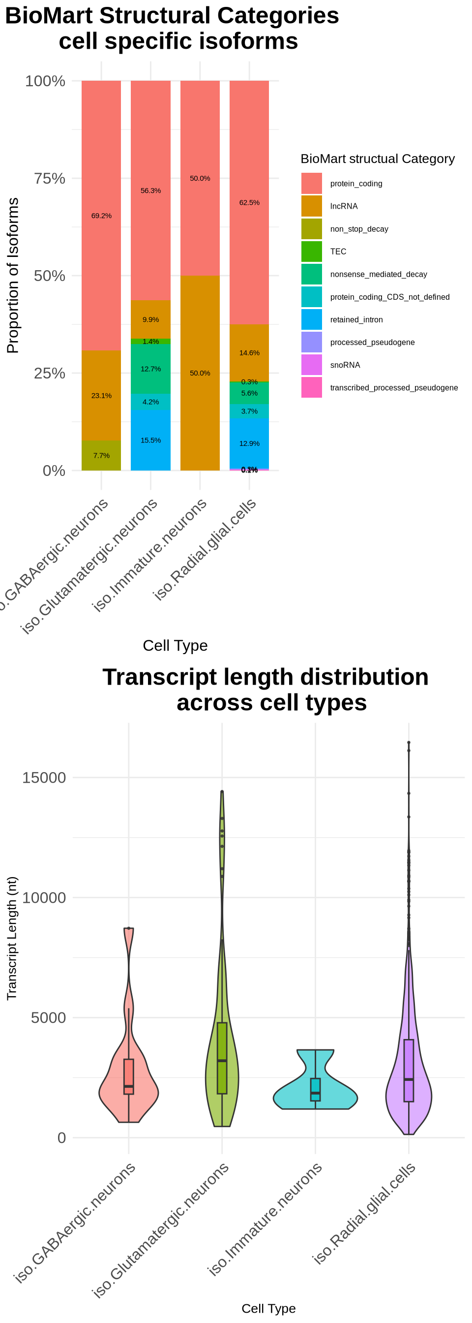
For more detail about the classification system see the SQANTI publication.↩︎
It is essential to keep in mind that cell type classification, sequencing depth, and the number of cells in each cluster can significantly impact the results, especially in cases where isoforms are expressed at very low levels.↩︎