Chapter 10 Multisample analysis

The FLAMES pipeline supports the analysis of multiple samples simultaneously, allowing users to handle more complex experimental designs without having to process each sample independently. This is implemented through the FLAMES::MultiSampleSCPipeline() function, which produces outputs that are analogous to the single-sample workflow described in earlier chapters, but extends it to multi-sample experiments and ensures that novel isoform discovery is performed consistently across the entire dataset.

To take full advantage of these features, we first need to perform a few initial processing steps:

Sample QC – Basic preprocessing and quality control are largely the same as for a single sample. Here, we also show how to start directly from FLAMES output and perform initial QC without empty droplet removal or ambient RNA normalisation. These extra steps are recommended, but may not always be required depending on the dataset.
Sample integration – Combining multiple samples into a single integrated object to remove batch effects and align shared biological structure.
Adding isoform counts – Incorporating isoform-level counts into the integrated Seurat object so that gene- and isoform-level analyses can be performed side by side.
Cell type identification – Annotating the integrated object with biologically meaningful cell type labels.

In this chapter, we will walk through these steps using a small subset of a multi-sample dataset (described below). Once we have an integrated object that contains both gene and isoform counts, we can use it as the foundation for a range of downstream analyses. In the following chapters, we will illustrate two key examples:

Trajectory analysis – using pseudotime to identify genes and isoforms that change along differentiation paths.
Differential transcript usage (DTU) analysis – investigating changes in isoform proportions between conditions.

10.0.1 Dataset Information

For this analysis, we use a subset of the neuronal differentiation dataset described in Wang et al. (2025). The full dataset contains eight samples spanning four time points from an excitatory neuronal differentiation protocol. To keep the tutorial runtime manageable, we randomly selected 2000 cells in total drawn from four samples at the first two timepoints: two stem cell (STC) samples and two Day 25 samples. This subset still captures the early stages of neuronal differentiation and allows us to explore temporal changes in gene and isoform expression between stem cells and early neuronal progenitors.

10.1 Standard pre-processing and quality control

As before we will modify the count matrix for each sample so we use gene_symbol instead of ENSGID. The data generated from this multisample experiment is quite large. This is especially the case with Oarfish isoform quantification as there are many more features to consider. This means much of the workflow below is time consuming and computationally intensive. Please keep this in mind when processing your samples. In the tutorial we provide code for the required steps but do not evaluate many of the sections below due to these computational constraints. The raw counts are available in the multisample data folder if users wish to run through the analysis.

First we will make the isoform gene dictionary for the mutisample mode.

Code

# The FLAMES ref can be found in your selected output folder after running the Flames pipeline. 
FLAMES_gtf_file <- "data/multi_sample_subset/isoform_annotated.gtf" #ensure file is unzipped
reference_gtf_file <- "data/gencode.v47.annotation.gtf" # ensure file is unzipped
output_file <- "isoform_gene_dict_mutlisample_subset.csv"

# Call the helper function defined in code block above to create a dictionary containing corresponding gene information for each isoform
# This may take a few minutes 
isoform_gene_dict_mutlisample <- make_isoform_gene_symbol_dict(FLAMES_gtf_file,
                                                   reference_gtf_file,
                                                   output_file)

Code

# convert Gene_id to gene symbol for all counts
#run a loop to run this function on all count files.
# Directory with input files
input_dir <- "./data/multi_sample_subset/"
output_dir <- "./data/multi_sample_subset/"

# List all CSV files in the input directory
input_files <- list.files(input_dir, pattern = "\\count_subset.csv$", full.names = TRUE)

# Initialize an empty list to store data frames
result_list <- list()

# Process each file in the directory
total_files <- length(input_files)  # Total number of files

for (i in seq_along(input_files)) {
  file_path <- input_files[i]
  
  # Extract file name without extension
  file_name <- tools::file_path_sans_ext(basename(file_path))
  
  # Construct the output file name
  output_file <- file.path(output_dir, paste0(file_name, "_gene_symbol.csv"))
  
  # Show progress to the user
  message(sprintf("Processing file %d of %d: %s", i, total_files, file_name))
  
  # Call the function with return_df = TRUE to store the result
    result_list[[file_name]] <- convert_ENSGID_to_geneSymbol(
    id_symbol_df = isoform_gene_dict_mutlisample,
    gene_count_matrix_path = file_path,
    output_file = output_file,
    return_df = TRUE
  )
}

## Processing file 1 of 4: C1_STC_matched_reads_gene_count_subset

## Processing file 2 of 4: C2_Day25_matched_reads_gene_count_subset

## Processing file 3 of 4: C4_STC_matched_reads_gene_count_subset

## Processing file 4 of 4: C5_Day25_matched_reads_gene_count_subset

10.1.1 Define QC function

We have developed a multisample QC function @ref(Multisample QC function) for processing count matrices and constructing filtered Seurat objects, following best practices outlined in the Seurat tutorial. This function includes steps to identify and remove doublets, as well as generate key diagnostic plots for data inspection. We encourage users to customize this function to fit their specific needs, such as applying additional filtering criteria.

For the purposes of presenting concise and readable code we will apply the default filtering parameters to all objects. If users wish to be more specific about filtering each sample independently this is possible and can be done by running the perform_qc_filtering function on each sample with desired parameters.

Code

# Define sample names
sample_names <- c("C1_STC", "C4_STC", "C2_Day25", "C5_Day25")

# Initialize a list to store UMAP objects
umap_objects <- list()

# Start the PDF for output
pdf(file = "./output_files/multi_sample_subset/QC/multisample_QC.pdf", width = 10, height = 6)

# Loop through each sample and apply the QC filtering function
for (i in seq_along(sample_names)) {
  sample_name <- sample_names[i]
  
  # Print progress message
  message(paste0("Processing sample ", i, " of ", length(sample_names), ": ", sample_name))
  
  # Perform QC filtering
  result <- perform_qc_filtering(
    result_list[paste0(sample_name, "_matched_reads_gene_count_subset")],
    fig_name = sample_name,
    project = sample_name
  )
  
  # Store the UMAP object from the result
  umap_objects[[sample_name]] <- result[[1]]
}

# Close the PDF device
dev.off()

#save the object
#saveRDS(umap_objects, file = "./output_files/multi_sample_subset//umap_objects.rds")

10.2 Multisample integration

First we will merge the Seurat objects together and then perform integration. There are many options for sample integration and Seurat provides many wrappers for these functions. Here we will use Harmony (Korsunsky et al., 2019) for fast and effective integration. The code chunk bellow takes our samples and merges them together.

Code

# integrate samples  
#from the function above pull the filtered seurat object 
umap_objects <- readRDS("./output_files/multi_sample_subset//umap_objects.rds")

merged_seurat <- merge(
  umap_objects[["C1_STC"]],
  y = list(
    umap_objects[["C4_STC"]],
    umap_objects[["C2_Day25"]],
    umap_objects[["C5_Day25"]]
  ),
  add.cell.ids = c(
    "C1_STC", "C4_STC", "C2_Day25", "C5_Day25"
  ), 
  project = "Multi-sample_tutorial"
  )

# create a sample column
merged_seurat$sample <- rownames(merged_seurat@meta.data)

## split sample column to make a batch col
merged_seurat@meta.data <- separate(merged_seurat@meta.data, col = 'sample', into = c('batch', 'Day', 'Barcode'), 
                                    sep = '_')
#check some QC metrics 
VlnPlot(merged_seurat, features = c("nFeature_RNA", "nCount_RNA", "percent.mt"), ncol = 3, group.by = "Day") + 
  plot_annotation(title = "Vln plots grouped by Day")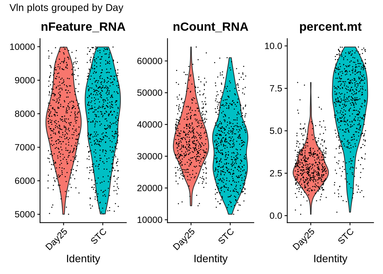

Code

#can plot based on any metadata col
#VlnPlot(merged_seurat, features = c("nFeature_RNA", "nCount_RNA", "percent.mt"), ncol = 3, group.by = "orig.ident")

# Number of cells per group
table(merged_seurat$orig.ident)

## 
##   C1_STC C2_Day25   C4_STC C5_Day25 
##      225      330      328      138

Code

table(merged_seurat$Day)

## 
## Day25   STC 
##   468   553

Code

# Apply normal preprocessing steps to merged file 

merged_seurat <- NormalizeData(object = merged_seurat)

## Normalizing layer: counts.C1_STC

## Normalizing layer: counts.C4_STC

## Normalizing layer: counts.C2_Day25

## Normalizing layer: counts.C5_Day25

Code

merged_seurat <- FindVariableFeatures(object = merged_seurat)

## Finding variable features for layer counts.C1_STC

## Warning in simpleLoess(y, x, w, span, degree = degree, parametric = parametric, : pseudoinverse used at -2.0512

## Warning in simpleLoess(y, x, w, span, degree = degree, parametric = parametric, : neighborhood radius 0.30103

## Warning in simpleLoess(y, x, w, span, degree = degree, parametric = parametric, : reciprocal condition number
## 2.3467e-16

## Finding variable features for layer counts.C4_STC

## Warning in simpleLoess(y, x, w, span, degree = degree, parametric = parametric, : pseudoinverse used at -2.2148

## Warning in simpleLoess(y, x, w, span, degree = degree, parametric = parametric, : neighborhood radius 0.30103

## Warning in simpleLoess(y, x, w, span, degree = degree, parametric = parametric, : reciprocal condition number
## 4.1338e-16

## Finding variable features for layer counts.C2_Day25

## Finding variable features for layer counts.C5_Day25

## Warning in simpleLoess(y, x, w, span, degree = degree, parametric = parametric, : pseudoinverse used at -1.8388

## Warning in simpleLoess(y, x, w, span, degree = degree, parametric = parametric, : neighborhood radius 0.30103

## Warning in simpleLoess(y, x, w, span, degree = degree, parametric = parametric, : reciprocal condition number
## 5.5033e-16

Code

merged_seurat <- ScaleData(object = merged_seurat)

## Centering and scaling data matrix

Code

merged_seurat <- RunPCA(object = merged_seurat)

## PC_ 1 
## Positive:  L1TD1, MGST1, GRID2, CACNA2D3, PRDX1, MT-CO3, HSPA8, GALNT17, POLR3G, ADGRV1 
##     ENSG00000248605, MT-ATP6, RBFOX1, ROR1, SHISA9, GPR176, RBM47, MT-CO2, SNTG2, PTPRG 
##     BNC2, SPATS2L, ENSG00000274090, HDAC2-AS2, MCM3, MT-CYB, FRAS1, ENSG00000203279, RPL22L1, CALN1 
## Negative:  MALAT1, ENSG00000280441, ENSG00000278996, DACH1, ENSG00000280614, ENSG00000280800, ZEB1, ENSG00000281181, SOX5, TUBA1A 
##     DLK1, ENSG00000257060, ENSG00000281383, WNT5B, NNAT, MAP2, ZFHX4, MEIS2, GPM6A, NPAS3 
##     MAPK10, CKB, FGF13, KCNQ3, ZBTB20, GREB1L, VIM, SSBP2, SOX6, LINC01414 
## PC_ 2 
## Positive:  ENSG00000259316, HMGB2, RPS24, SOX2-OT, VIM, DEK, CENPH, HMGN2, PTTG1, TUBA1B 
##     H2AZ2, CDC20, BIRC5, FRZB, LINC01830, MIR99AHG, LIX1, MXD3, H2AX, SMC4 
##     RPS3A, TYMS, CCNB2, MT-ND3, UBE2C, PBK, NUSAP1, ENSG00000285920, CCN1, IGFBP2 
## Negative:  RIMS2, STMN2, AKAP6, NFASC, XKR4, NALF1, CHN2, RMST, GAP43, KIF5C 
##     PCSK2, NRXN1, ANK3, PTPRD, ERC2, CADPS, NSG2, MYT1L, CACNA2D1, ENSG00000283982 
##     LINC01917, CTNNA2, ELAVL2, PBX1, CELF3, SLIT1, INA, DST, ELAVL4, CACNA1B 
## PC_ 3 
## Positive:  JPT1, TUBB2A, TMSB10, UBE2S, RBP1, S100A11, CRABP1, TUBB, BDNF-AS, NEFM 
##     PLAAT3, S100A10, TUBB2B, STMN2, ID2, DYNLL1, INA, IGFBPL1, MT1X, GDAP1L1 
##     GNG8, ST18, GAP43, CELF3, ID3, INSM1, TAGLN, PCSK1N, NSG2, LDHA 
## Negative:  GPC6, FBXL7, B3GALT1, FAT3, DLG2, ENSG00000228222, QKI, EFNA5, PLEKHA5, PARD3B 
##     XYLT1, TOX, NRG3, LINC03077, STK3, NLGN1, PTPRK, KCNT2, SDK1, EXT1 
##     GRIP1, RAD51B, PRKD1, DAB1, LDB2, SUPT3H, CDK14, TTC28, NAV3, KIAA1217 
## PC_ 4 
## Positive:  DANT2, RPL22L1, RPS24, BDNF-AS, RPS3A, PCDH11X, ENSG00000271860, MT-RNR2, PLAAT3, PRKG1 
##     TPM1, MT-CO3, DANT1, S100A11, ADAMTS6, ENSG00000272449, BST2, MT1X, LINC01414, DIAPH2 
##     MT-RNR1, DGKB, RPL34, ENSG00000289195, MT-CO1, ENSG00000239920, ATP2B4, USP38-DT, ID3, ENSG00000297419 
## Negative:  PBK, NUSAP1, PRC1, TOP2A, NUF2, ENSG00000285920, MXD3, TPX2, GAS2L3, NEK2 
##     CENPA, HMGB2, MKI67, KIF18A, CKAP2L, CDCA3, TUBB4B, KIF2C, FAM72C, GTSE1 
##     SGO2, KIFC1, CENPE, FAM72A, H2AX, FAM72D, ASPM, CDCA8, NDC80, RACGAP1 
## PC_ 5 
## Positive:  CDH18, LINC02609, LHX5-AS1, TBR1, EBF1, RSPO3, GPR149, SLC4A10, ENSG00000286446, SLIT1 
##     ENSG00000296399, SLC17A6, FSTL5, EPB41L3, ANKFN1, ROBO1, PCSK2, LHX1-DT, ENSG00000293110, LHX5 
##     PCDH9, TRH, EPHA3, ENSG00000227681, SAMD5, PCSK1N, GABBR2, RORB, ENSG00000259316, ENSG00000224658 
## Negative:  ASCL1, RASD1, DLX6-AS1, GADD45G, RGS16, NRXN3, MEST, NXPH1, GAD2, SMOC1 
##     COPG2IT1, ENSG00000258416, SOX4, COPG2, DLL1, SLCO5A1, GNG8, LINC02106, ENSG00000258637, MYT1 
##     ATP2B4, ENSG00000234710, PXDN, RND3, TH, ENSG00000295572, NOL4, ENSG00000270953, ISL1, PCP4

Code

merged_seurat <- FindNeighbors(object = merged_seurat, dims = 1:16)

## Computing nearest neighbor graph

## Computing SNN

Code

merged_seurat <- FindClusters(object = merged_seurat, resolution = 0.6)

## Modularity Optimizer version 1.3.0 by Ludo Waltman and Nees Jan van Eck
## 
## Number of nodes: 1021
## Number of edges: 29966
## 
## Running Louvain algorithm...
## Maximum modularity in 10 random starts: 0.8700
## Number of communities: 8
## Elapsed time: 0 seconds

Code

merged_seurat <- RunUMAP(object = merged_seurat, dims = 1:30)

## 12:41:32 UMAP embedding parameters a = 0.9922 b = 1.112

## 12:41:32 Read 1021 rows and found 30 numeric columns

## 12:41:32 Using Annoy for neighbor search, n_neighbors = 30

## 12:41:32 Building Annoy index with metric = cosine, n_trees = 50

## 0%   10   20   30   40   50   60   70   80   90   100%

## [----|----|----|----|----|----|----|----|----|----|

## **************************************************|
## 12:41:32 Writing NN index file to temp file /tmp/RtmpSqzgLk/file35f6113b834dc
## 12:41:32 Searching Annoy index using 1 thread, search_k = 3000
## 12:41:32 Annoy recall = 100%
## 12:41:34 Commencing smooth kNN distance calibration using 1 thread with target n_neighbors = 30
## 12:41:36 Found 2 connected components, falling back to 'spca' initialization with init_sdev = 1
## 12:41:36 Using 'irlba' for PCA
## 12:41:36 PCA: 2 components explained 51.16% variance
## 12:41:36 Scaling init to sdev = 1
## 12:41:36 Commencing optimization for 500 epochs, with 39318 positive edges
## 12:41:38 Optimization finished

Code

##save merged object
saveRDS(merged_seurat, file = "./output_files/multi_sample_subset//merged_seurat.rds")

We then integrate the samples using Harmony and generate UMAPs from both the merged (non-integrated) and integrated data. This allows us to visually compare how well integration has reduced sample-specific batch effects. In this dataset, the integrated UMAP shows that cells from different samples cluster together based on their biological state rather than their sample of origin, indicating that there is no obvious sample-driven bias in the clustering.

Code

set.seed(00003)
merged_seurat <- readRDS("./output_files/multi_sample_subset/merged_seurat.rds")


#Let's plot the merged file. 
p1 <- FeaturePlot(merged_seurat, reduction = 'umap', features = 'nCount_RNA')
p2 <- FeaturePlot(merged_seurat, reduction = "umap", features = 'nFeature_RNA')
p3 <- DimPlot(merged_seurat, reduction = 'umap', group.by = 'Day')
p4 <- DimPlot(merged_seurat, reduction = 'umap', group.by = 'orig.ident')

grid.arrange(p1, p2, p3, p4, ncol = 2)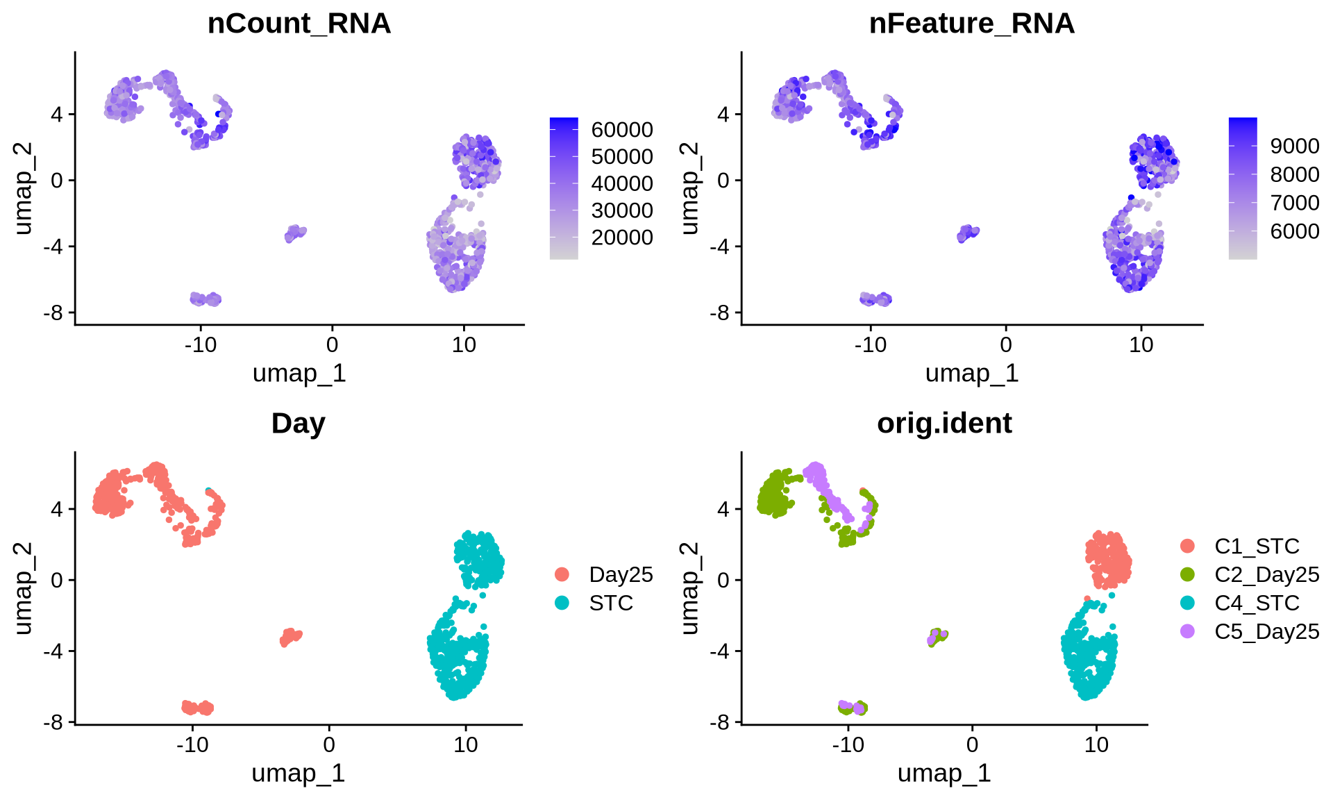

Code

merged_seurat <- JoinLayers(object = merged_seurat)
merged_seurat[["RNA"]] <- split(merged_seurat[["RNA"]], f = merged_seurat$orig.ident)

#perform integration with Harmony
obj <- IntegrateLayers(object = merged_seurat,
                       method = HarmonyIntegration,
                       orig.reduction = "pca",
                       new.reduction = 'integrated.harm',
                       verbose = FALSE,
)

## Warning in harmony::HarmonyMatrix(data_mat = Embeddings(object = orig), : HarmonyMatrix is deprecated and will be removed in the
## future from the API in the future

Code

obj <- FindNeighbors(obj, reduction="integrated.harm")
obj <- FindClusters(obj, resolution=0.4, cluster.name="harm_cluster")

## Modularity Optimizer version 1.3.0 by Ludo Waltman and Nees Jan van Eck
## 
## Number of nodes: 1021
## Number of edges: 29472
## 
## Running Louvain algorithm...
## Maximum modularity in 10 random starts: 0.8720
## Number of communities: 7
## Elapsed time: 0 seconds

Code

obj <- RunUMAP(obj, reduction="integrated.harm", dims=1:50, reduction.name = "umap.harm")


DimPlot(obj, reduction = "umap.harm", group.by = c("Day", "orig.ident", "harm_cluster"), label = T)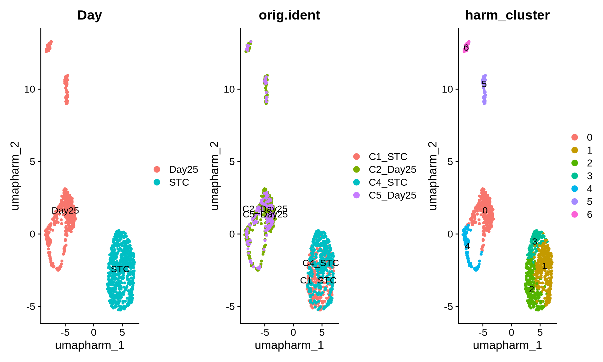

Code

### save object 
saveRDS(obj, file = "./output_files/multi_sample_subset//integrated_harm_seurat.rds")

10.3 Add isoform counts

Now we can add isoform level information to the integrated Seurat object. When doing this you may need to convert the Oarfish files into a count.csv file with the row names in the ENSTID_genesymbol form. The function to do so can be found here @ref(Convert Oarfish files to count matrix). The function also allows you to include or exclude novel bambu genes quantified by Oarfish; for the sake of simplicity in this tutorial, we will exclude these novel bambu genes.

Code

# Define sample names
sample_names <- c("C1_STC",
                  "C4_STC",
                  "C2_Day25",
                  "C5_Day25")

# Loop through each sample and process the count files
for (sample in sample_names) {
  # Use tryCatch to handle errors
  tryCatch({
    # Call the function to process the sample
    process_oarfish_files_to_counts_matrix(
      sample_name = sample,
      resource_table_path = "./output_files/ref_files/isoform_gene_dict_mutlisample_subset.csv",
      output_dir = "./output_files/multi_sample_subset/oarfish_counts/",
      input_dir = "./data/multi_sample_subset/oarfsih/",
      filter_bambu_Genes = TRUE
    )
  }, error = function(e) {
    # Print the error message and exit the loop
    cat("Error processing sample:", sample, "\nError message:", e$message, "\nExiting loop.\n")
    stop(e)
  })
}

Once we have created the CSV files with the correct structure (ENSTID_genesymbol), we can add the isoform information back into our gene-level object. First, we create an isoform-level Seurat object for each sample and merge these into a single isoform Seurat object. Next, we filter the merged isoform object to retain only high-quality cells, using the cell types and QC filters defined in the gene-level analysis above.

Code

############ read in count matrix and add isoform assay to Seurat object  #########
#Make Seurat objects not filtered
# Function to read a CSV file and create a Seurat object
create_seurat_object <- function(sample_name, input_dir, project_name) {
  # Construct file path
  file_path <- file.path(input_dir, paste0("gene_symbol_oarfish_", sample_name, "_counts.csv"))
  
  # Read the CSV file
  counts <- fread(file_path)
  counts <- as.data.frame(counts) 
  rownames(counts) <- counts[[1]]            # Set row names from the first column
  counts[[1]] <- NULL     
  
  # Create the Seurat object
  seurat_obj <- CreateSeuratObject(counts = counts, project = project_name, min.cells = 5, min.features = 500)
  
  return(seurat_obj)
}

# Directory where the CSV files are stored
input_directory <- "./output_files/multi_sample_subset/oarfish_counts/"

# Create an empty list to store Seurat objects
iso_seurat_objects <- list()

total_samples <- length(sample_names)
for (i in seq_along(sample_names)) {
  sample <- sample_names[i]
  
  message(sprintf("Processing sample %d of %d: %s", i, total_samples, sample))
  
  iso_seurat_objects[[sample]] <- create_seurat_object(
    sample_name = sample,
    input_dir = input_directory,
    project_name = sample
  )
}

####### Merge the samples into one object ######
iso.merged_seurat <- merge(
  iso_seurat_objects[["C1_STC"]],
  y = list(
    iso_seurat_objects[["C4_STC"]],
    iso_seurat_objects[["C2_Day25"]],
    iso_seurat_objects[["C5_Day25"]]
  ),
  add.cell.ids = c(
    "C1_STC", "C4_STC", "C2_Day25", "C5_Day25"
  ), 
  project = "iso-Multi-sample_tutorial"
  )

# create a sample column
iso.merged_seurat$sample <- rownames(iso.merged_seurat@meta.data)

# split sample column to makw a batch col
iso.merged_seurat@meta.data <- separate(iso.merged_seurat@meta.data, col = 'sample', into = c('batch', 'Day', 'Barcode'), 
                                    sep = '_')

## filter the data to iso and gene cells match
merged_seurat_isoform_filtered <- subset(iso.merged_seurat, cells =obj@graphs[["RNA_nn"]]@Dimnames[[1]])

VlnPlot(merged_seurat_isoform_filtered, features = c("nFeature_RNA", "nCount_RNA", "percent.mt"), ncol = 3)

# perform standard workflow steps
merged_seurat_isoform_filtered <- NormalizeData(object = merged_seurat_isoform_filtered) # if using SCT dont run this
merged_seurat_isoform_filtered <- FindVariableFeatures(object = merged_seurat_isoform_filtered) # if using SCT dont run this
merged_seurat_isoform_filtered <- ScaleData(object = merged_seurat_isoform_filtered) # if using SCT dont run this
merged_seurat_isoform_filtered <- RunPCA(object = merged_seurat_isoform_filtered)
#ElbowPlot(merged_seurat_isoform_filtered)
merged_seurat_isoform_filtered <- FindNeighbors(object = merged_seurat_isoform_filtered, dims = 1:10)
merged_seurat_isoform_filtered <- FindClusters(object = merged_seurat_isoform_filtered, resolution = 0.6)
merged_seurat_isoform_filtered <- RunUMAP(object = merged_seurat_isoform_filtered, dims = 1:10)

#Save file
saveRDS(merged_seurat_isoform_filtered, file = "./output_files/multi_sample_subset//merged_seurat_isoform_filtered.rds")

We can then add this merged isoform object as a new assay in the gene-level Seurat object, allowing gene- and isoform-level analyses to be performed side by side. In principle, the isoform assay could also be integrated across samples (e.g. using Harmony) to further remove sample-specific batch effects, but for simplicity we do not perform isoform-level integration in this tutorial and rely on gene level integration.

Code

merged_seurat_isoform_filtered <- readRDS(file = "./output_files/multi_sample_subset//merged_seurat_isoform_filtered.rds")

#plots
p5 <- DimPlot(merged_seurat_isoform_filtered, reduction = 'umap', group.by = 'orig.ident')
p6 <- DimPlot(merged_seurat_isoform_filtered, reduction = 'umap', group.by = 'Day')
p7 <- FeaturePlot(merged_seurat_isoform_filtered, reduction = 'umap', features = 'nCount_RNA')
p8 <- FeaturePlot(merged_seurat_isoform_filtered, reduction = "umap", features = 'nFeature_RNA')

grid.arrange(p5, p6, p7, p8, ncol = 2)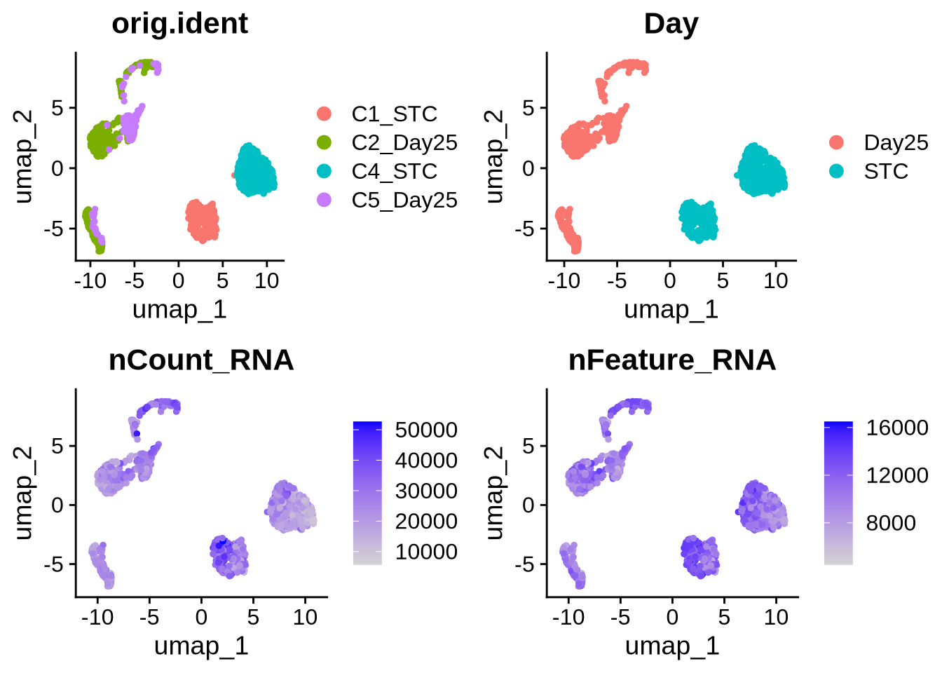

Code

#####

merged_seurat_isoform_filtered <- JoinLayers(merged_seurat_isoform_filtered)
counts_table <- merged_seurat_isoform_filtered[["RNA"]]$counts

obj[["iso"]] <- CreateAssay5Object(counts = counts_table)

# Step 1: Normalize the new assay data
obj <- NormalizeData(obj, assay = "iso")
obj <- FindVariableFeatures(obj, assay = "iso")
obj <- ScaleData(obj, assay = "iso")

# Step 4: Perform PCA
obj <- RunPCA(obj, assay = "iso", reduction.name = "pca_iso")

## Warning: Key 'PC_' taken, using 'pcaiso_' instead

Code

# Step 5: Run UMAP
obj <- RunUMAP(obj, reduction = "pca_iso", dims = 1:15, assay = "iso", reduction.name = "umap_iso")

# Visualize the UMAP
DimPlot(obj, label = TRUE, reduction = "umap.harm") | DimPlot(obj, label = TRUE, reduction = "umap_iso")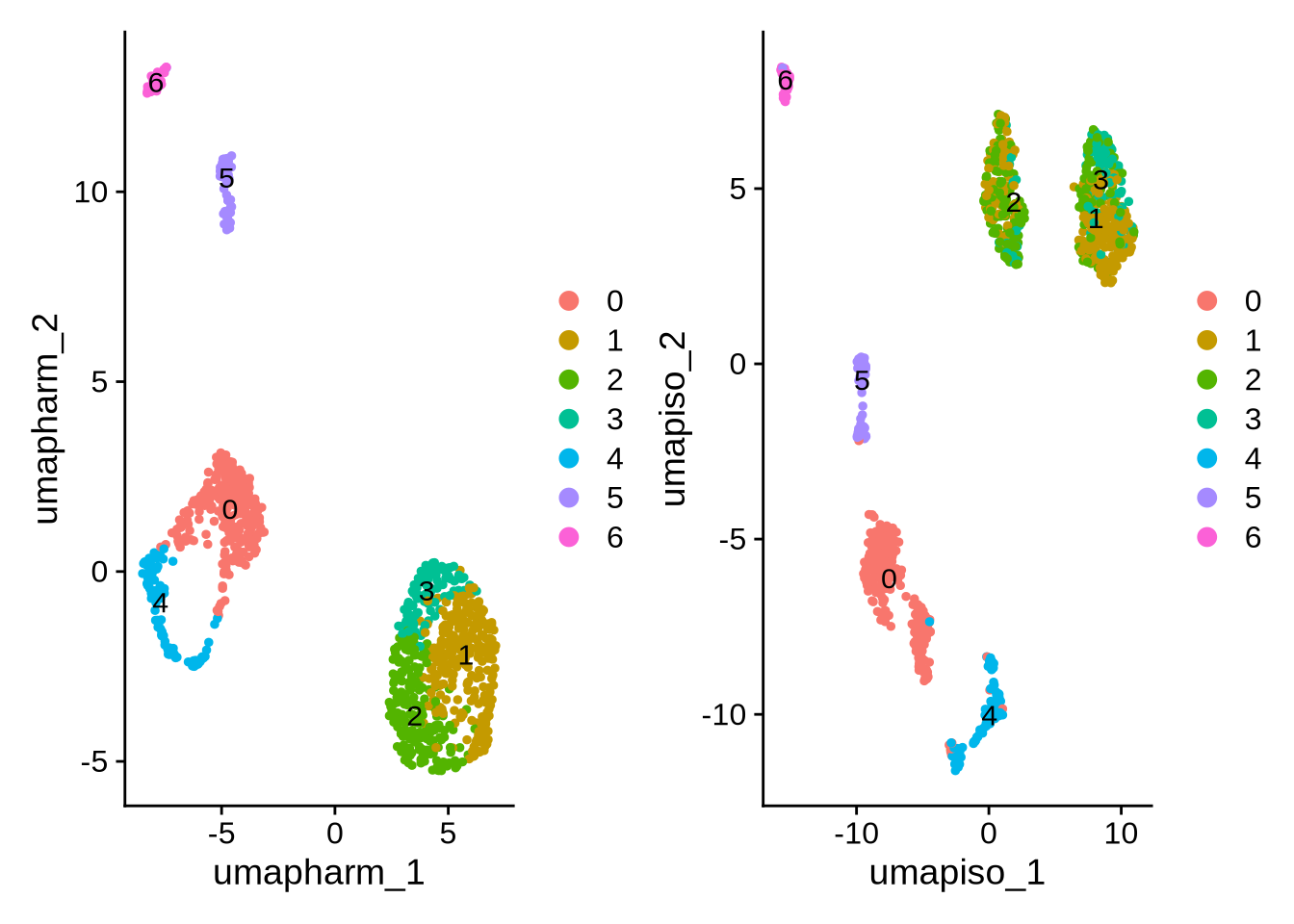

Now we have a complete object to work with that contains an integrated gene-level assay and isoform counts for the same set of cells. As with any single-cell analysis, the next step is to annotate cell types, so that downstream analyses can be interpreted in a biologically meaningful way.

10.4 Identify cell types

Here, we annotate cell types using a small set of key marker genes. We keep this step deliberately simple, as automated annotation methods and GO-enrichment-based strategies have already been described in earlier chapters.

Cluster 1 2 and 3 are stem ells

Code

# We can annoate Day 0 
FeaturePlot(obj, reduction = "umap.harm", features = c("MKI67", "NANOG", "POU5F1"), ncol = 3)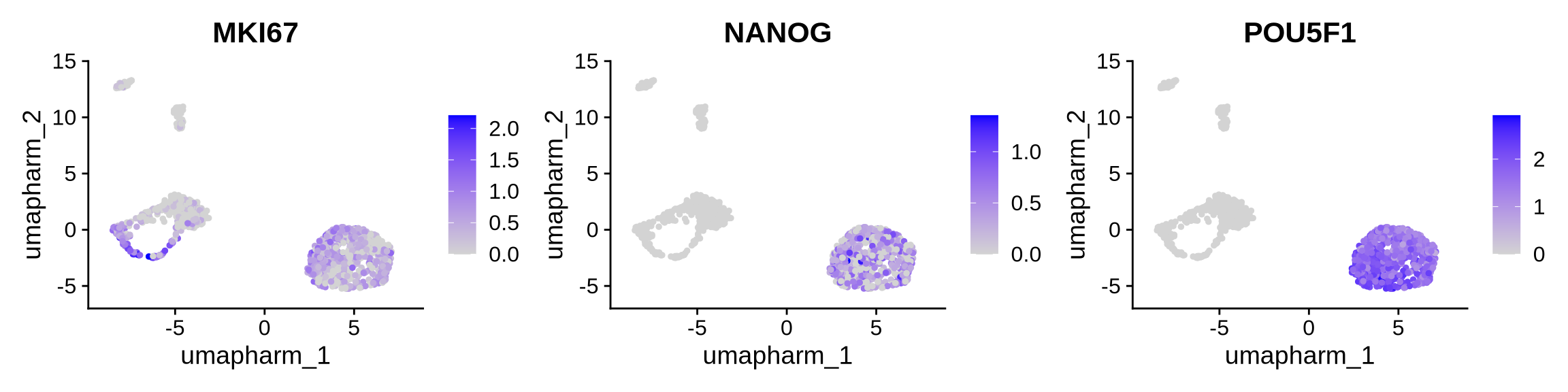

Cluster 0 and 4 - Radial Glia

Code

FeaturePlot(obj, reduction = "umap.harm", features = c("VIM", "SOX2", "PAX6"), ncol = 3)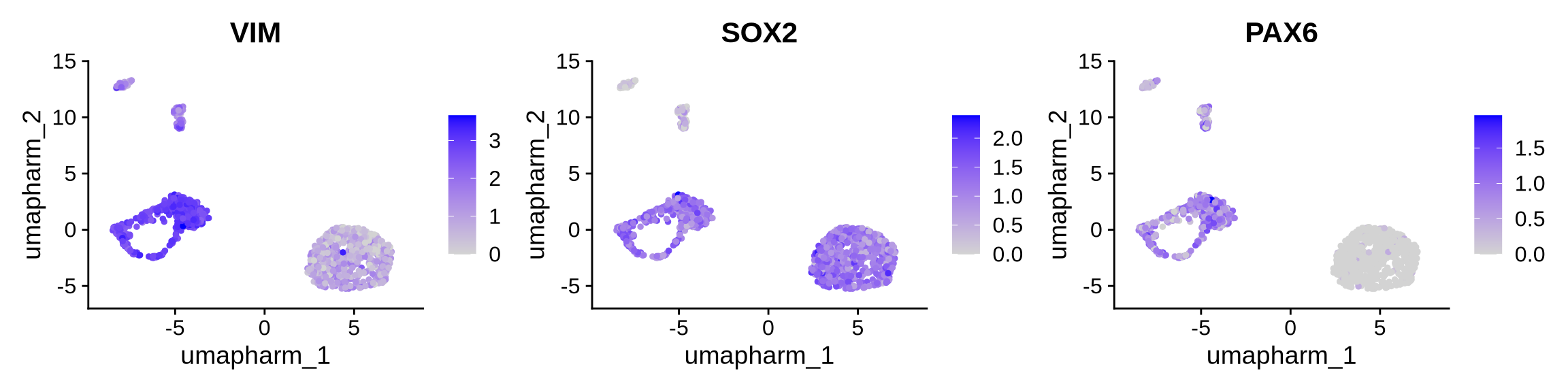

Cluster 5 - Inhibitory neurons

Code

FeaturePlot(obj, reduction = "umap.harm", features = c("GAD1", "GAD2", "DLX5", "DLX6"),ncol = 4)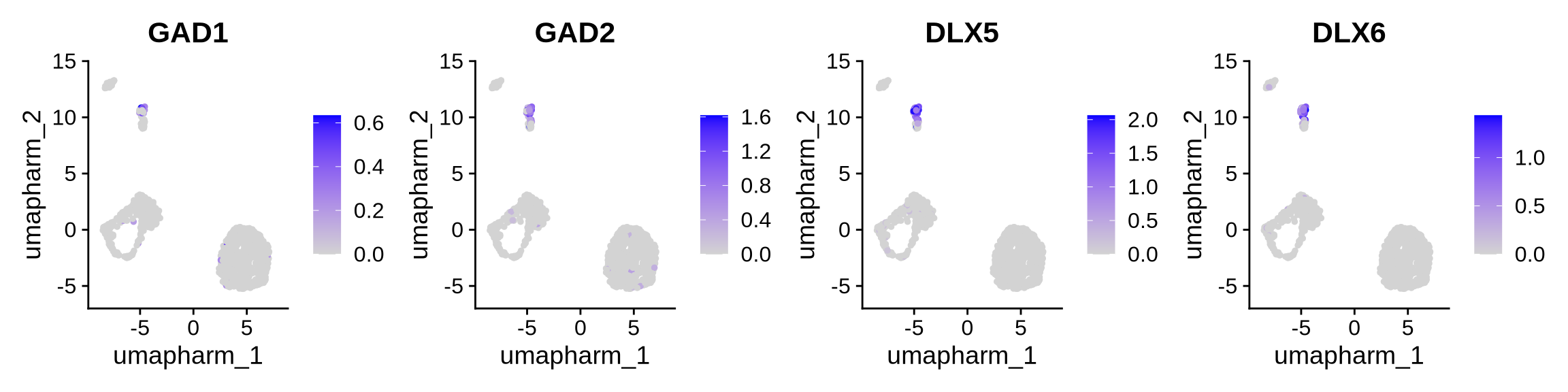

Cluster 6 - Excitatory neurons (NPC)

Code

#Clsuter 6 Excitorty neurons (NPC)
FeaturePlot(obj, reduction = "umap.harm", features = c("EOMES", "TBR1"))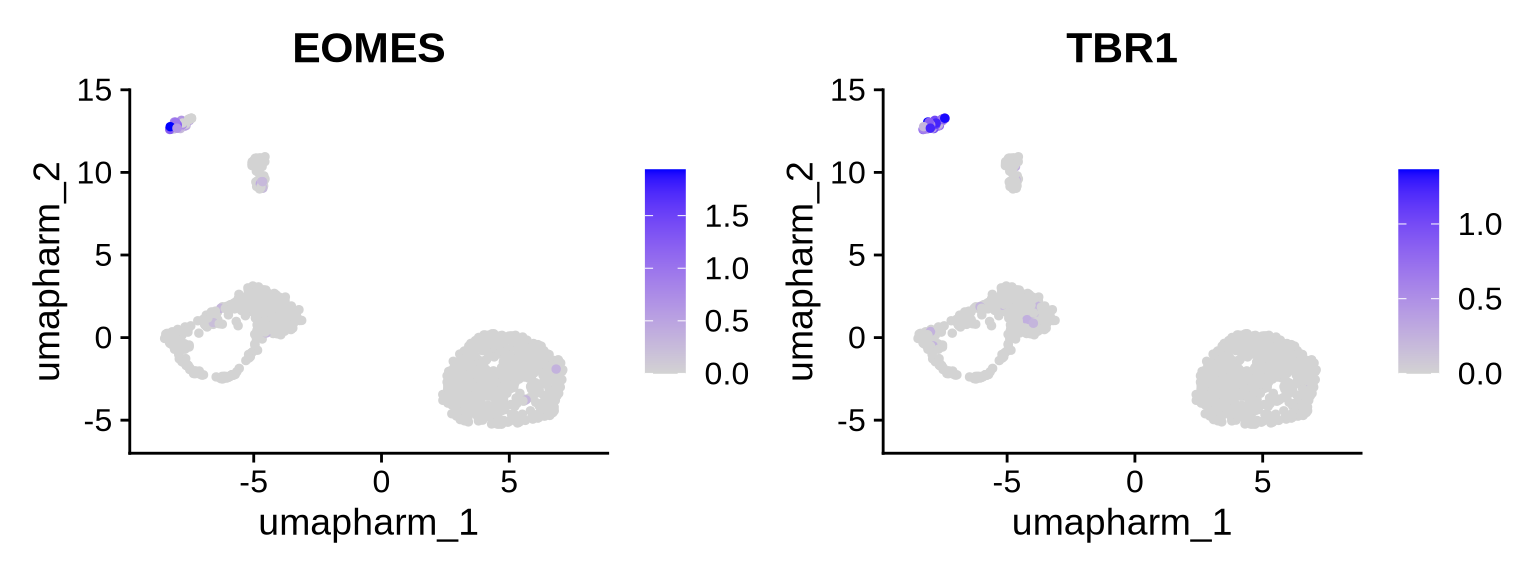

Now we will assign these labels to each cluster.

Code

new_ids <- c(
  "0" = "Radial glia",
  "1" = "Stem cells",
  "2" = "Stem cells",
  "3" = "Stem cells",
  "4" = "Radial glia",
  "5" = "Inhibitory neurons",
  "6" = "Excitatory neurons"
)

obj <- RenameIdents(obj, new_ids)

# store as a metadata column for later
obj$cell_type <- Idents(obj)

# plot by cell type instead of numeric cluster
DimPlot(obj, group.by = "cell_type", reduction = "umap.harm")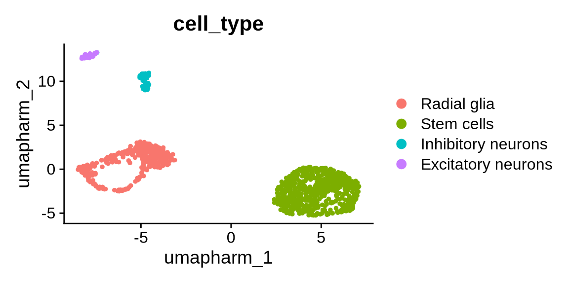

Code

#saveRDS(obj, file = "./output_files/multi_sample/multisample_seurat.intergrated_harm.isoform.rds")

Now that we have an integrated Seurat object containing both gene- and isoform-level counts, along with curated cell type annotations, we can move beyond static clustering to explore how these transcriptional programs change over time and across lineages. In the next sections, we will use this object as the foundation for trajectory analysis, to reconstruct developmental paths and cell state transitions, and for differential transcript usage (DTU) analysis, to identify genes whose isoform composition shifts between conditions, lineages, or cell types.